Run the whole pipeline

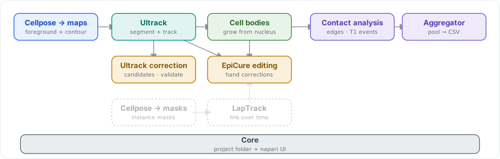
itasc[all] ships the dense pipeline end to end: Cellpose maps, Ultrack, cell bodies, both correction tools, and the contact and aggregate stages. The sparse Cellpose-masks path is a separate tool. Solid chips are shipped; dashed are the rest of the family.

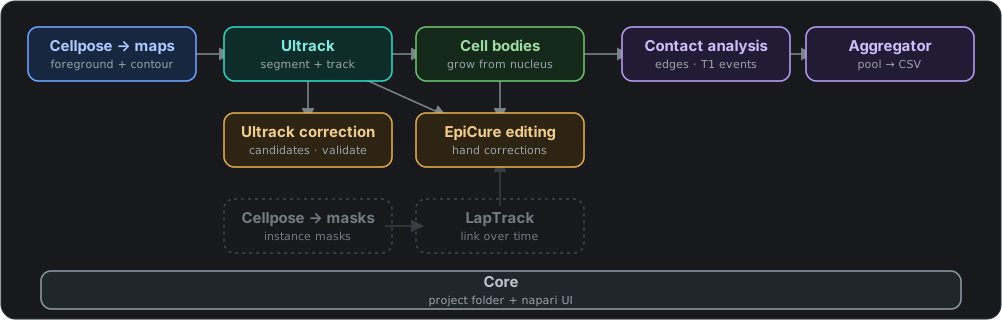
itasc[all] ships the dense pipeline end to end: Cellpose maps, Ultrack, cell bodies, both correction tools, and the contact and aggregate stages. The sparse Cellpose-masks path is a separate tool. Solid chips are shipped; dashed are the rest of the family.

itasc[all] is the full plugin: the whole pipeline in one napari widget, segment, track, correct, and quantify, in that order, without leaving the viewer. Reach for it when you have dense, motile cells of varying shape and want to go from raw stacks to quantified contacts in one place.

One idea holds the app together: every stage writes its result to disk, and the next stage reads that result back. The project folder is the source of truth. You can inspect it between stages, resume from any point, or hand a single stage to its standalone distribution.

Install

uv tool install napari --with "itasc[all]"

The [all] extra pulls the core scientific stack plus the two workflow engines it imports and runs: Cellpose-SAM (cellpose, torch, torchvision) and the Ultrack solver. If you have never installed Python before, the install guide walks through it from an empty machine and covers GPU setup, updating, and removal. From a local checkout, for development:

python -m pip install -e ".[all]"

The project on disk

The folder is the source of truth, so it is worth knowing its shape. ITASC expects a project directory with one subdirectory per position (pos00, pos01, …). Within a position, each stage reads the files the previous stage wrote and writes its own into the next folder:

pos00/
  0_input/              raw prepared input stacks
  1_cellpose/           Cellpose probability and flow outputs, divergence maps
  2_nucleus/            nucleus segmentation, Ultrack database, tracked labels
  3_cell/               cell segmentation and tracked labels
  nucleus_labels.tif    committed nucleus tracked labels
  cell_labels.tif       committed cell tracked labels
  contact_analysis.h5   contact graph built from the committed labels

The numbered folders hold re-runnable working artifacts. The committed labels and the contact_analysis.h5 built from them sit together in the position root. Everything is plain files, so you read the state of a run by looking at the folder: an empty 3_cell/ means cell segmentation has not run yet.

A full run, stage by stage

Start napari and open the plugin:

napari
# then: Plugins > ITASC > ITASC

The ITASC panel docks on the right. Its sections run top to bottom in the same order as the stage folders on disk: Cellpose, Nucleus Segmentation & Tracking, Cell Segmentation, Contact Analysis. Each section acts on the current position and writes into its stage folder. The screens below walk one position from raw stacks to quantified contacts.

Point the plugin at your data

Open a project folder with Project at the top of the panel, set the pixel size and frame length, and name the nucleus and cell input stacks. The panel writes this to itasc_config.json in the project, so the metadata travels with the data and reloads next time.

To try the app before you have data of your own, download itasc-sample-data.zip (12 MB) and point it at the unzipped sample_data/ folder: it holds the same three positions shown on this page. If you cloned the repository, it is already there, in sample_data/.

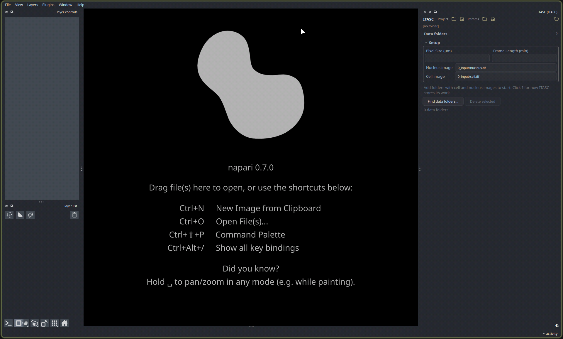
The panel before any folder is added: pixel size, frame length, and the names of the nucleus and cell input stacks.

Find data folders… scans the project for positions and lists them. Each position carries a status rail, one dot per stage: a hollow dot for not started, amber while a stage runs, green once its output is committed, red when that output is stale. Click a dot to load that stage’s output into the viewer. The stage sections appear below once at least one folder is present, each collapsed and ready to run. Run all contact analyses runs the final contact-analysis stage across every listed position at once. That is the only stage that runs start to finish without a person: Cellpose, tracking, and segmentation each need a human at the wheel, tracking correction most of all, so they run one position at a time. The sections below walk that single-position pass and show what each stage produces.

Running a stage never loads anything. Every stage writes its result to the project folder and stops there, so a pass of Run · Run · Run · Run leaves the layer list exactly as you left it. Opening something is always your own move: a stage’s rail dot, a row in its Pipeline Files panel, Visualize Contact Analysis, or entering correction mode. The live previews inside each stage are the exception that proves the rule — they put layers up because looking at them is the whole point of a preview. The figures below show what each stage produces once it has been loaded that way.

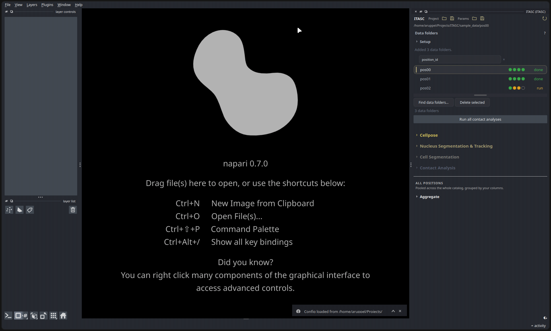
Three positions found. The stage sections below, one per folder on disk, run top to bottom.

Stage 1: Cellpose

Cellpose finds the cells. This section runs the nucleus and cell channels through Cellpose-SAM to write probability and flow (dp) maps under 1_cellpose/, then reduces those to the foreground and contour maps that seed tracking and segmentation. Preparing the input maps explains what the two maps are and how they are built from Cellpose’s output. The Pipeline Files list at the top of every section is the ledger: inputs check off, outputs fill in as they are written.

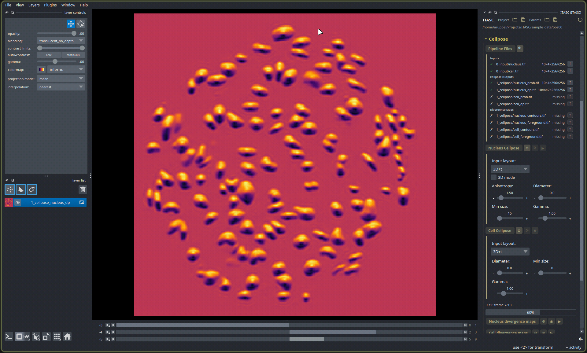
Cellpose mid-run. The nucleus maps are written and checked; the cell maps are still missing. The viewer shows a nucleus divergence map.

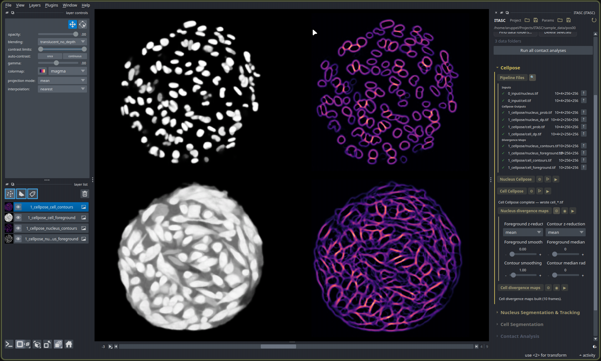
Cellpose finished. Contour and foreground maps for both channels: every later stage reads these, never the raw stacks.

Stage 2: Nucleus segmentation and tracking

This section (standalone: itasc-tracking) turns the nucleus maps into tracked labels under 2_nucleus/. Segmentation and tracking are solved together, not one after the other: this is the Ultrack model. Outlining and tracking the nuclei explains why that matters and what the solver is doing; the steps below are how you drive it.

Atom extraction breaks the nucleus foreground into atoms: the smallest fragments an oversegmentation splits it into. Run writes 2_nucleus/atoms.tif; turn the live preview on to watch the fragments while you tune the parameters.

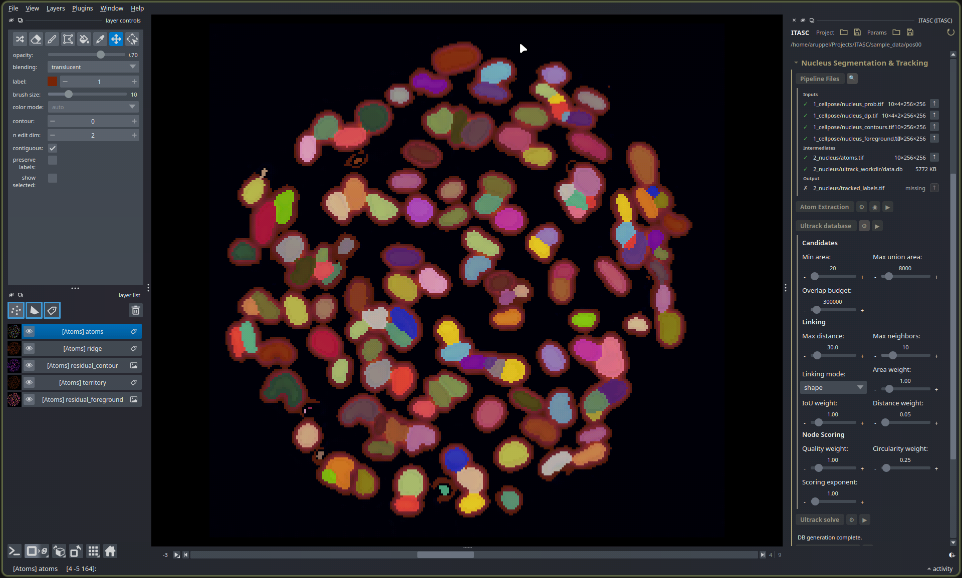
Atom extraction with the live preview on. The [Atoms] layers hold the fragments every later candidate is built from.

Ultrack database assembles those atoms into every plausible merge, so one nucleus may appear as a single atom, a pair, or a larger clump. Each merge is a candidate segmentation, and all of them, across all frames, go into one database.

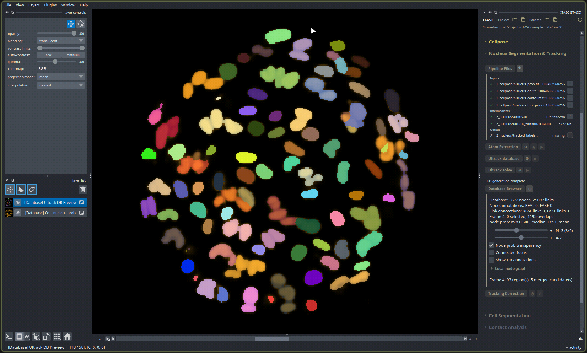
The candidate database: 3672 nodes, 29097 links. The browser inspects one frame’s candidates before a solve.

Ultrack solve then picks one candidate per nucleus per frame and links the picks across frames in a single optimization, trading off the event penalties and solver settings so the labels are coherent in time rather than decided frame by frame. The result is 2_nucleus/tracked_labels.tif: one label per track, held across every frame. Click the nucleus stage’s rail dot to open it as a Tracked: Nucleus layer, or go straight into correction, which loads it for you.

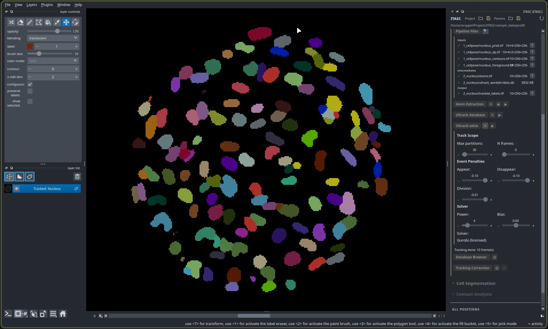
Solved tracks: one color per nucleus, held across all ten frames.

Correct the tracks

No solver is perfect on dense, dividing cells, so the tracks get a human pass, and the correction widget runs on the same candidate database. Its candidate gallery surfaces the database’s stored alternatives for the selected nucleus, so most fixes are a click on a candidate the solver did not pick rather than a redraw from scratch.

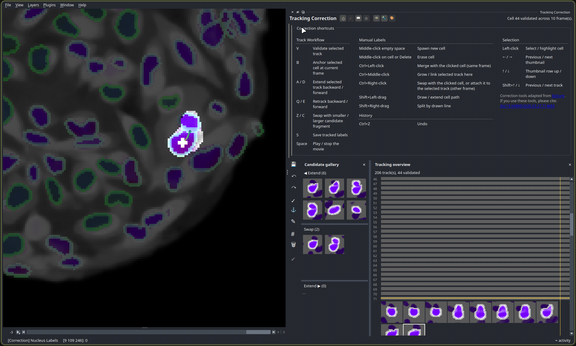
Tracking Correction: the shortcut reference, the candidate gallery for the selected nucleus, and the per-track overview, 44 of 206 tracks validated.

The tools fall into three kinds:

• Manual. Merge two cells, spawn a new cell, split a cell, or redraw its contour by hand.

• Semi-manual. Pull a bigger or smaller candidate for the selected nucleus, stepping up or down its merge hierarchy in the database.

• Tracking fixes. Swap two labels, retrack a track locally, or extend the current track into the next frame from a database candidate.

Some of these tools are adapted from EpiCure. Work through the tracks and validate as you go; the overview turns green for every track confirmed.

A corrected track scrubbed across frames: the selected nucleus stays anchored while the overview fills green for every frame it is validated across.

Stage 3: Cell segmentation

Cells grow out from the tracked nuclei. This section builds a weighted cost field from the cell contour and foreground maps and cuts it into cell territories, writing tracked cell labels to 3_cell/. The nuclei are already tracked, so each cell inherits the track ID of the nucleus it grew from: nucleus and cell share an identity for free. Growing the cell bodies covers why the bodies follow the nuclei rather than being tracked themselves. As with the nuclei, a correction step follows, the same tools in the same interactive layer, to fix merged or split cells before the labels are committed.

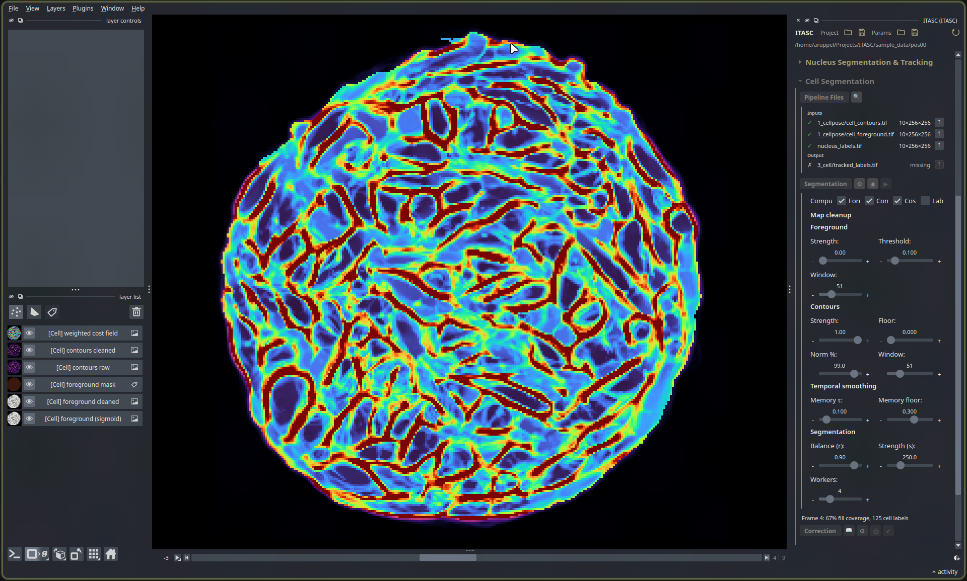
The weighted cost field, built from the cell contour and foreground maps. Segmentation cuts this into territories.

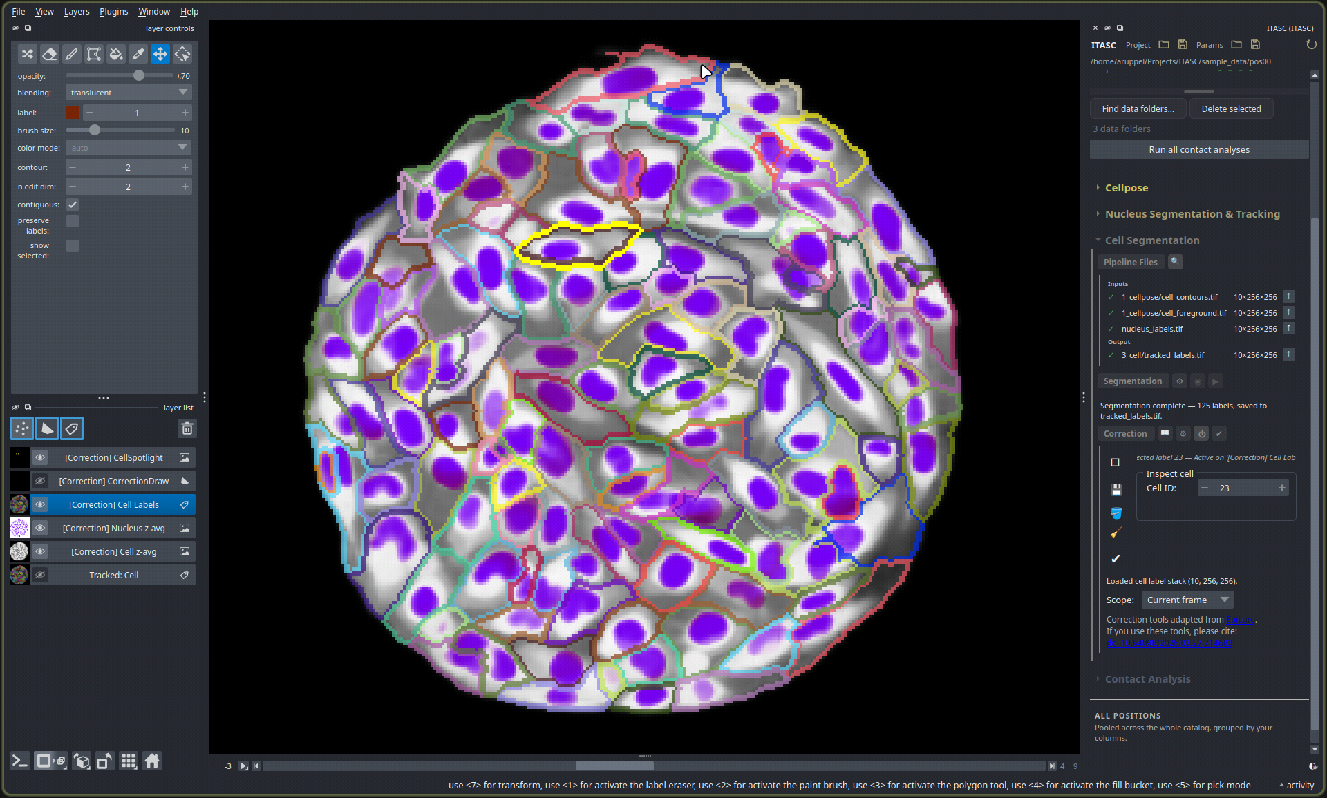
Segmentation finished: 125 cell labels, outlines over the nucleus channel, with the correction panel open below. Inspect cell isolates one label to check it.

Stage 4: Contact analysis

The last stage reads the committed nucleus and cell labels and writes contact_analysis.h5 to the position root: the contact graph, the shared edges between neighbors, and the T1 events where two neighbors swap partners. The two buttons split the work cleanly: Run Contact Analysis rebuilds the .h5 and touches nothing in the viewer, Visualize Contact Analysis loads the result back as napari layers (building it first if it isn’t there yet).

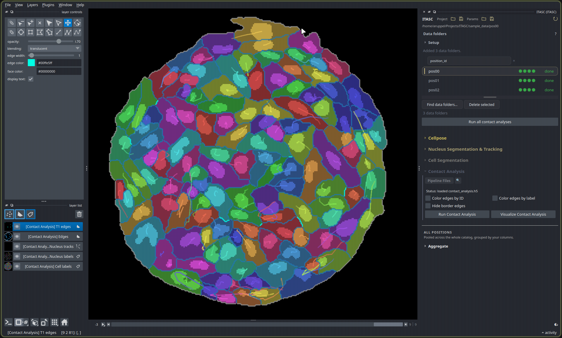
The contact analysis loaded back: cell labels, nucleus tracks, contact edges, and the T1 edges where a contact forms or breaks.

Aggregate across positions

Everything so far runs one position at a time. Aggregate (standalone: itasc-aggregate) is the one section that reaches across the whole project: it reads every position’s contact_analysis.h5 and pools the results into project-level tables, one CSV per quantity. Tick the quantities to pool, cell density, cell and nucleus shape, neighbor count, contact length, and the rest, then Pool ready positions writes them to the project root.

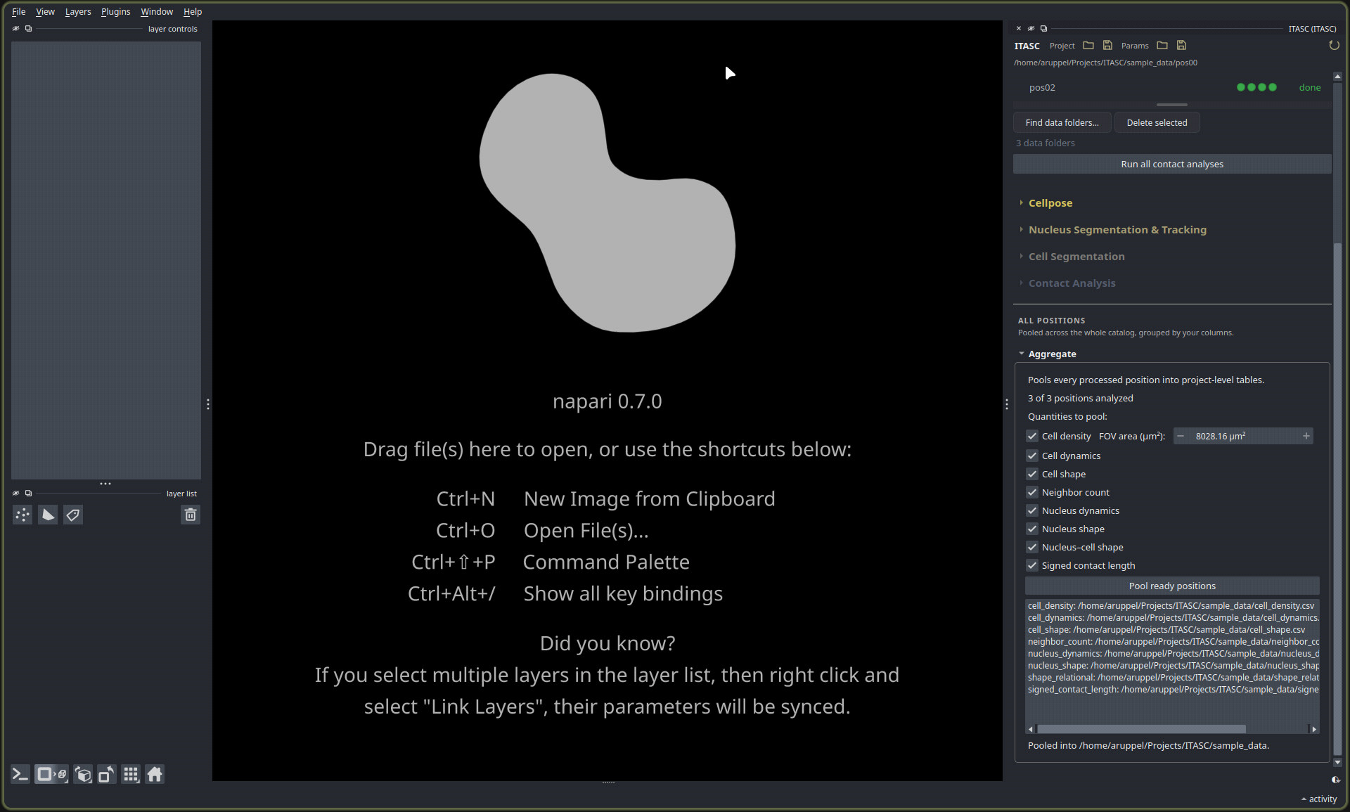
Aggregate over all three positions. Each ticked quantity becomes one CSV in the project root, ready for stats and plots outside napari.

The aggregate guide covers what each table holds and how to run it on its own.

Start from a later stage

If your data already sits partway down the pipeline, skip ahead. Foreground and contour maps let you start at nucleus tracking; tracked cell labels let you start at contact analysis. Each stage also ships as a standalone distribution for running it on its own data: the distribution overview maps each entry point to its distribution.

This tour stays at the level of what each section does. Each stage has a guide of its own that goes deeper into its parameters and standalone use: Cellpose, nucleus tracking, and aggregation.