Outlining and tracking the nuclei

This stage turns the two nucleus maps into tracked nuclei: for every nucleus, an outline in each frame and one identity that holds across the whole movie. It implements the approach described in the overview: rather than committing to a single outline per frame, multiple candidate outlines are built, and a single optimization selects the set that is most consistent in time.

The stage proceeds in three steps. The maps are cut into small pieces called atoms. The atoms are grouped into candidate outlines, and each possible correspondence between a candidate in one frame and a candidate in the next is scored. A solver then selects, across all frames simultaneously, a consistent set of outlines and links. Remaining errors are corrected manually.

The stage operates only on the nucleus maps. Cell bodies are generated in a later stage from this result.

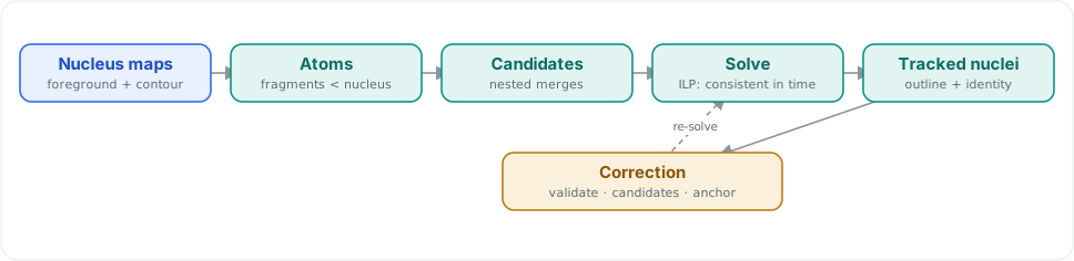
The four steps: the maps are cut into atoms, the atoms are merged into candidate outlines, a solver selects a consistent set across time, and the result is corrected. Correction feeds back into the solver, which re-solves with the confirmed tracks held fixed.

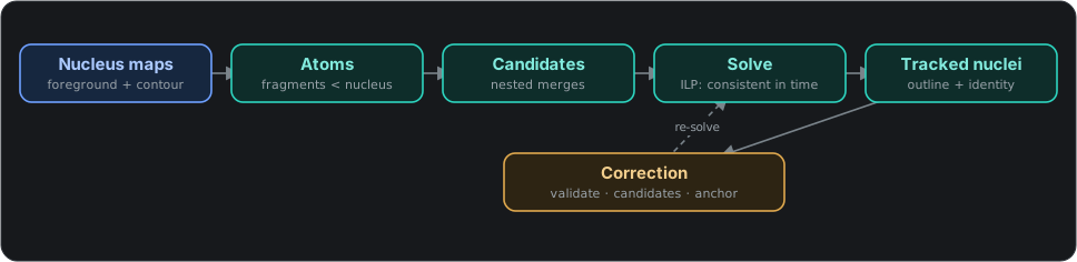
The four steps: the maps are cut into atoms, the atoms are merged into candidate outlines, a solver selects a consistent set across time, and the result is corrected. Correction feeds back into the solver, which re-solves with the confirmed tracks held fixed.

Atoms

An atom is a fragment smaller than a nucleus, or at most equal to one. The foreground is cut into atoms along the ridges of the contour map: the map is flooded inward from the center of each nucleus, and the floods meet at the ridges between nuclei. Each nucleus therefore corresponds to a group of whole atoms rather than a partial atom. Over-marking boundaries in the previous stage is acceptable for this reason: an extra ridge splits one atom into two, which grouping can recombine, whereas a missing ridge merges two nuclei into atoms that cannot later be separated.

Before the cut, the local background of each map is subtracted, so that a single brightness threshold separates nucleus from background across the whole frame rather than only in regions where the image is bright.

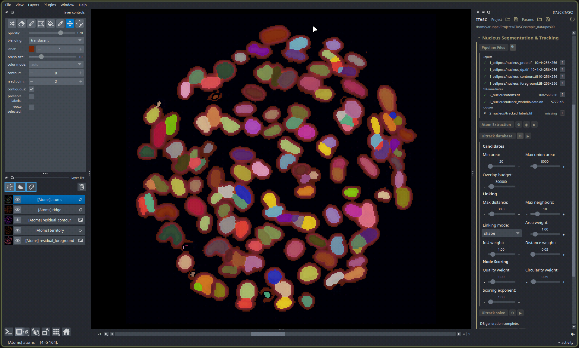
The sample nuclei cut into atoms, in the main canvas: each nucleus is one or a few colored tiles, and the dark ridges between tiles fall on the boundaries. The panel on the right holds the settings described in this page.

The Atom Extraction panel controls the cut. The values listed below are those configured for the example data and used on a first run. For other images, Min area and the two window sizes are the parameters most likely to require adjustment, as they are measured in pixels.

Setting	What it does	Default
FG window	The size, in pixels, of the neighborhood averaged to estimate the local background of the foreground map.	51
FG cutoff	How bright a point must be, after that background is subtracted, to count as part of a nucleus.	0.002
FG strength	How much of the local background to subtract: 1 removes all of it, 0 removes none.	1
Contour window	The same neighborhood size for the contour map.	20
Contour floor	How strong a ridge must be to act as a wall between atoms. Lower values cut along fainter boundaries.	0.05
Contour strength	How much of the contour map’s local background to subtract before the ridges are read.	0.16
Min area	The smallest atom to keep, in pixels. A smaller fragment is folded into the neighbor with which it shares the longest border.	10

Candidates

A nucleus may correspond to a single atom, a pair, or a small clump. Rather than selecting one grouping, the stage generates all plausible groupings as candidate outlines. Candidates are built by merging atoms across their weakest walls first, so that each merge is the next most probable one, and every intermediate grouping is retained as a candidate. Selection among the candidates occurs in the solver step.

Atoms merging into candidate outlines. Fragments belonging to one nucleus share a color and are combined into that nucleus’s outline, the merge proceeding across the weakest boundaries first.

Candidates are then linked across time. For each candidate in a frame, the candidates in the next frame that could correspond to the same nucleus are identified, and each such link is assigned a similarity score. The score is a weighted sum of three terms: the agreement in size between the two outlines (weighted by Area weight), their overlap (weighted by IoU weight), and the distance between their centers (weighted by Distance weight). The first two terms are rewards and the third is a penalty, so a pair of similar outlines lying close together scores higher than a distant or dissimilar pair.

Overlap is measured after the later outline is shifted so that its center coincides with that of the earlier one, so that translation between frames does not by itself reduce it; only differences in shape and size do. Motion is accounted for separately by the distance term, the raw separation between the two centers in pixels. The resulting scores are read by the solver to follow a nucleus from frame to frame.

These settings are located under the Ultrack database step, divided into the Candidates, Linking, and Node Scoring groups. The defaults are tuned to the example data and rarely require changing. For other images, Max distance is the parameter to adjust first: it is a distance in pixels and must be at least as large as the distance a nucleus travels between two frames.

The Candidates group controls the outlines generated.

Setting	What it does	Default
Min area	The smallest candidate outline to keep, in pixels. Distinct from the atom Min area above: this parameter drops whole candidates, whereas that one folds away tiny fragments.	20
Max union area	The largest a candidate may grow to, in pixels. A limit on the number of atoms a single grouping may contain.	8000
Overlap budget	How many alternative groupings, beyond the most probable one, are retained as candidates. Higher values provide the solver with more candidates, at the cost of a larger and slower database.	300000

The Linking group scores the matches between frames.

Setting	What it does	Default
Max distance	The farthest, in pixels, a nucleus may travel between two frames and still be linked. Set above the fastest actual motion.	30
Max neighbors	The maximum number of candidates in the next frame considered as matches for one candidate.	10
Linking mode	shape scores a link by outline overlap, size, and distance. default uses Ultrack’s built-in linker.	shape
Area weight	How much a match in size contributes to a link’s score.	1
IoU weight	How much outline overlap contributes to a link’s score.	1
Distance weight	How much closeness contributes to a link’s score.	0.05

The Node Scoring group rates each candidate outline individually, before any link is considered, so that the solver can prefer clean, compact shapes.

Setting	What it does	Default
Quality weight	How much a candidate’s own quality contributes to its node score. Quality measures the intensity drop-off at the outline: the fraction of pixels in the ring just outside the candidate that are dimmer than its interior median, read from the Cellpose probability image. A candidate whose boundary sits on a clean edge scores near 1; one that bleeds into its surroundings scores low.	1
Circularity weight	How much a rounder outline is rewarded, nuclei being roughly round.	0.25
Scoring exponent	Sharpens the quality score: higher values widen the gap between good and poor candidates.	1

The solve

From the full database of candidates and links, the solver selects the set of outlines and links with the highest overall score, subject to two constraints derived from biology: two selected outlines may not share a pixel, and a nucleus may divide into two, while the reverse, two nuclei merging into one, is disallowed. Because an outline is selected together with the links that carry it through time, the selected outline is one that is also consistent with a track. The correct split of two touching nuclei is recovered in this way, as only that split remains consistent across the frames.

Without penalties, this scoring rule would create additional nuclei and divisions wherever doing so increases the total score. Three penalties constrain this: a fixed cost is applied each time a track starts, ends, or splits, so that these events occur only when supported by the image.

These settings are located under the Ultrack solve step and rarely require changing.

The Event Penalties are the three costs. Each is zero or negative; more negative values make the corresponding event less frequent.

Setting	What it does	Default
Appear	The cost of a track starting mid-movie. More negative values reduce the number of tracks that begin without a prior frame.	-0.1
Disappear	The cost of a track ending mid-movie.	-0.1
Division	The cost of one nucleus splitting into two. Near zero, so that genuine divisions are not strongly penalized.	-0.01

The Solver group controls the scoring and reports the engine in use.

Setting	What it does	Default
Power	How sharply outline overlap is rewarded: the overlap is raised to this power, so that a high value strongly favours nearly identical outlines from one frame to the next.	4
Bias	A constant offset added to every score, which shifts how readily the solver keeps a candidate. Reduce it when too many nuclei are kept, and increase it when too few are kept.	0
Solver	Read-only. Reports which mathematical engine solves the problem. Ultrack ships with the open-source CBC solver; if Gurobi is installed and licensed it is used instead. Gurobi requires a license (free for academic use), is much faster, and tends to find better solutions, so install it if you can.	—

The Track Scope group limits how much of the movie is solved, for running the pipeline on part of it. Set both to 0 to track the whole recording.

Setting	What it does	Default
N frames	How many frames to process. 0 processes all of them.	0 (all)
Max partitions	How many temporal windows to solve. 0 solves all.	0 (all)

Correction

On dense, dividing nuclei the solver output contains errors, and a single incorrect track affects every measurement derived from it. Correcting an entire movie cell by cell and frame by frame is impractical. Correction is therefore organized as an iterative process: the tracks are reviewed, correct tracks are confirmed, incorrect tracks are fixed, and the remainder is re-solved so that each fix propagates. Correction is applied only where the automatic result is incorrect, and confirmed work is not altered by subsequent re-solving.

The interface is a dedicated workspace: the movie on the left, a reference card of keyboard shortcuts, the candidate gallery, and a tracking overview that maps every track against every frame.

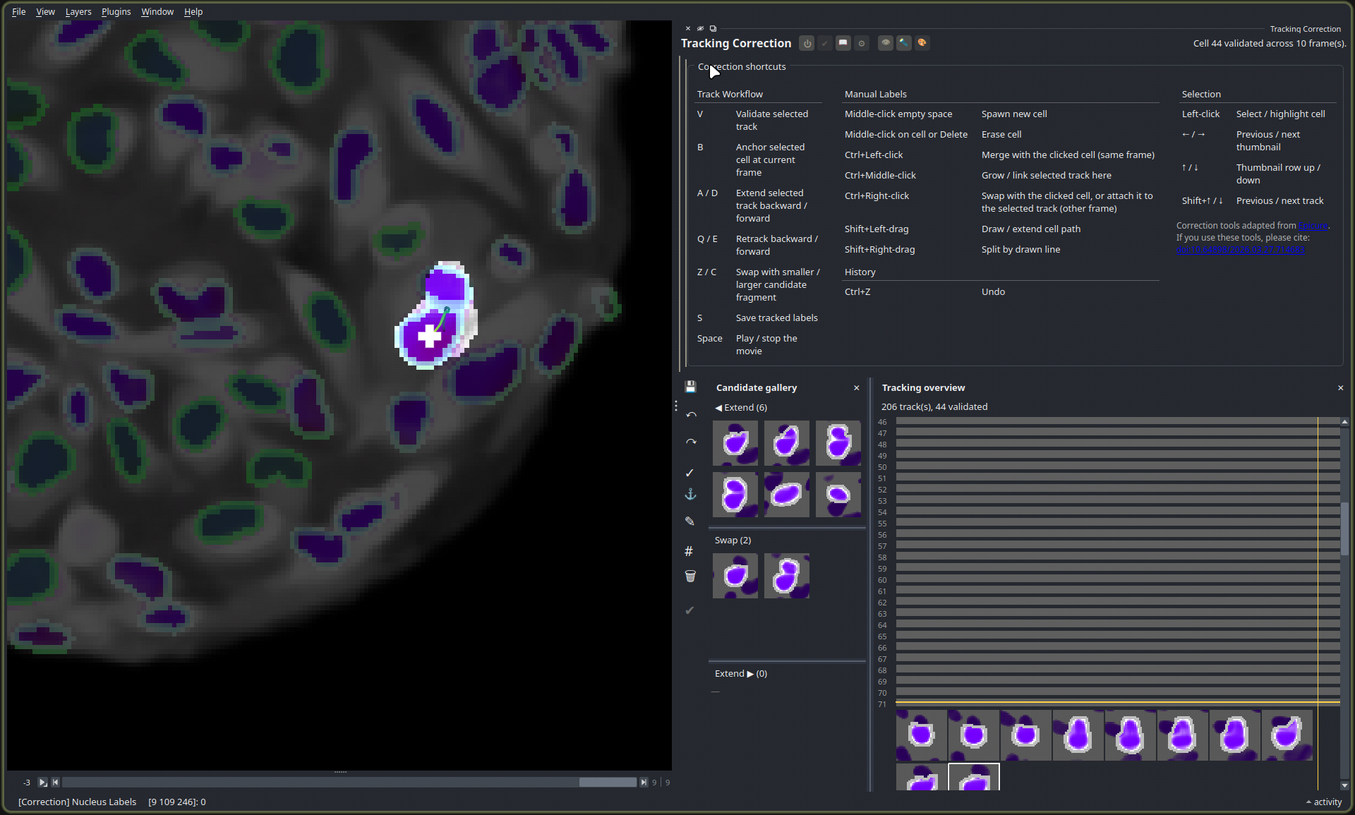
The correction workspace. One cell is selected (white, with its track path drawn through it) while the rest are dimmed. The right side lists the shortcuts, the candidate gallery provides alternative outlines, and the tracking overview reports how many of the 206 tracks are validated.

The workspace

The workspace is organized around keyboard operation and inspection of one track at a time.

The tracking overview displays every track as a row and every frame as a column, with validated stretches marked. Together with the counter (44 validated of 206 tracks), it indicates which tracks are complete and which remain. Selecting a track, either in the overview or in the image, displays a film strip along the bottom showing that track across all frames, in which an error appears as a break in the sequence. In the image, the selected cell is highlighted and the others are dimmed, and the cell’s track path is drawn as a line through the frames, indicating where the track deviates or jumps.

Selection and navigation use the keyboard: left-click selects a cell, ← and → step through the film-strip thumbnails, ↑ and ↓ move between rows, and Shift+↑ / Shift+↓ move to the previous or next track. Space plays the movie.

Review and validate

This step is the core of the correction process. Each track is reviewed against its film strip; if the outline and identity are consistent across all frames, V validates it. Validation locks the track and increments the counter, so that the overview is populated as review proceeds and the remaining work is indicated. A validated track is treated as ground truth and is not moved by subsequent re-solving.

The candidate gallery

When a track’s outline is incorrect, the correct outline is often among the candidates already generated. The solver retains the alternative outlines it built but did not select, and the gallery displays them as clickable thumbnails in three columns: Extend backward, Swap, and Extend forward. Clicking a Swap thumbnail replaces the current outline with that alternative; clicking an Extend thumbnail extends the track into the neighboring frame. From the keyboard, Z and C cycle the selected cell to the next smaller or larger candidate fragment, moving it up or down the merge tree of groupings built in the candidate stage.

Edit by hand

When no candidate is suitable, the labels are edited directly. These tools are adapted from EpiCure; cite it if you use them.

Gesture	What it does
Middle-click empty space	Spawn a new cell
Middle-click a cell, or Delete	Erase the cell
Ctrl+Left-click	Merge with the clicked cell, in the same frame
Shift+Left-drag	Draw or extend a cell’s outline
Shift+Right-drag	Split a cell along the drawn line
Ctrl+Middle-click	Grow or link the selected track to here
Ctrl+Right-click	Swap with the clicked cell, or attach it to the selected track across frames

Three cleanup actions adjust a mask after an edit: Fill Holes closes gaps inside a cell, Fix Semiholes closes near-enclosed indentations, and Clean Fragments removes stray specks carrying a cell’s label. Ctrl+Z undoes the last change.

Retrack and anchor

A correction to one frame is propagated to others by two independent tools.

Retrack operates from the currently selected cell. Q and E rerun the tracking backward or forward from the current frame: the current frame is used as the reference, and the unlocked cells in each neighboring frame are rematched to it in sequence, so that a correction propagates outward from the frame in which it was made. Validated tracks are not modified. A and D extend the selected track one frame at a time for manual growth.

Anchor pins a cell for a re-solve. B anchors the selected cell at the current frame, fixing it as a point that a full re-solve of the stack must honour there.

These tools support re-solving the whole movie: with correct tracks validated and locked, and difficult cells anchored, the entire stack can be re-solved, including with adjusted parameters, without altering the confirmed work. Correcting the least accurate tracks and re-solving is repeated until the result converges.

When the tracks are correct, S saves them. The corrected nucleus tracks are the output of this stage and the input to the next.

Where the tracks go

Each tracked nucleus now has an outline and an identity in every frame. The next stage, growing the cell bodies, uses these nuclei as seeds and extends a full cell body from each, so that every cell inherits the identity of its nucleus and the two remain aligned across the movie.