Measuring the result

This stage turns the corrected labels into numbers. It reads the tracked cell and nucleus labels the earlier stages produced and measures what the cells are and what they do: their shapes, their motion, which cells touch, and the moments neighbors swap. It runs in two steps. For each position, the cell-cell contacts and the neighbor-exchange events are found and written to one file. Across all positions, the per-cell measurements are pooled into tidy tables ready for statistics.

The stage measures; it does not interpret. The tables it writes carry no subpopulation classification and no plots: sorting cells into groups, reducing to replicate summaries, and drawing figures are downstream concerns, computed from these tables rather than inside this stage. This keeps the measurement one step and the interpretation another, so a later choice about how to group or plot the data does not reach back and change what was measured.

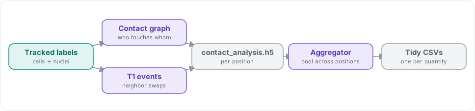
The two steps: per position, the tracked labels give a contact graph and its T1 events, written to one HDF5 file; then the aggregator pools every position into tidy CSV tables.

The two steps: per position, the tracked labels give a contact graph and its T1 events, written to one HDF5 file; then the aggregator pools every position into tidy CSV tables.

Cell-cell contacts

Two cells are in contact in a frame when their outlines share a boundary. That shared boundary is an edge, and its length is the length of the boundary between the two cells. Every edge in a frame, taken together, is the contact graph: which cells touch, and how long each junction is. A cell’s boundary against the image edge or the background is recorded separately as a border edge, so that a cell at the edge of the field is not mistaken for one fully surrounded by neighbors.

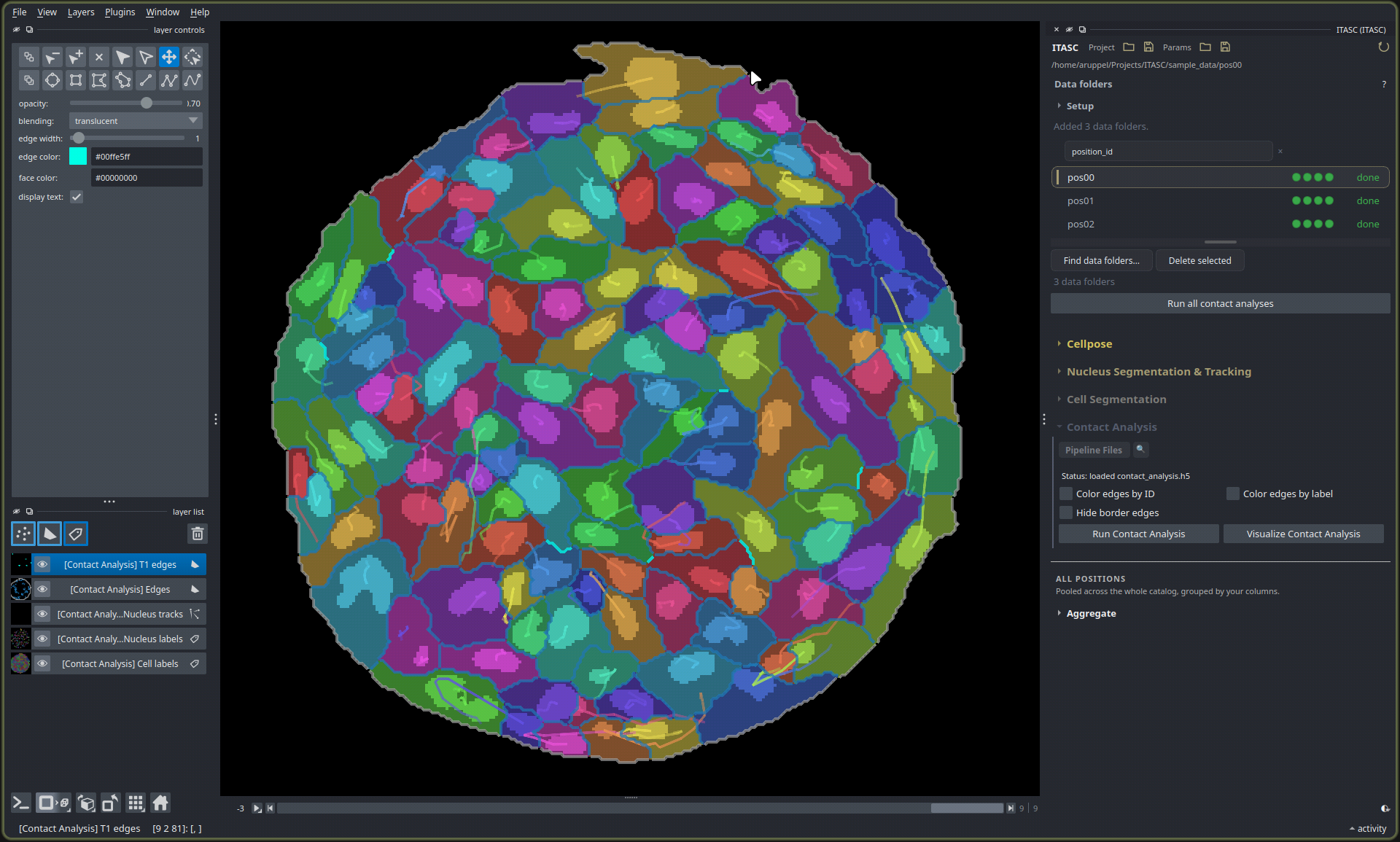
The contact graph for one frame, drawn over the cell labels: each cyan line is an edge, the shared boundary between two touching cells, with the edges involved in a neighbor swap highlighted. The panel on the right runs the analysis and controls this overlay.

The contacts are built once per position and written to a contact_analysis.h5 file holding the edges of every frame and the events described below. In the Contact Analysis panel, Run Contact Analysis builds this file for the current position and Run all contact analyses builds it for every position in the project. Visualize Contact Analysis draws the result back over the labels as an Edges layer and a T1 edges layer, and Color edges by ID, Color edges by label, and Hide border edges control that overlay.

Neighbor swaps

The elementary rearrangement of a monolayer is the T1 transition: a junction between two cells shrinks to a point and vanishes, and a new junction forms between the two cells that were kept apart by it. Four cells are involved: a losing pair, which were in contact and are separated, and a gaining pair, which were apart and come into contact.

A T1 event is found by comparing the contact graph between two consecutive frames. An edge present in the first frame and absent in the second is a candidate losing junction, and an edge absent then present is a candidate gaining junction. The two are recorded as one event when the four cells they name are distinct and each losing cell touches each gaining cell in both frames, which is the arrangement of four cells around a single vanishing junction. Each event is written with its losing pair, its gaining pair, the frame, and its location.

T1 events are the unit of tissue flow, so their rate and geometry are what a rearranging monolayer is measured by. One derived measurement is carried through to the tables: the signed length of the central junction across a swap, negative while the losing pair still touch and positive once the gaining pair do. The distribution of that signed length is a reaction coordinate whose inversion gives the effective energy barrier of the transition; that inversion, and the landscape it produces, are downstream of this stage.

Pooling across positions

Each analyzed position yields per-cell, per-frame measurements. The Aggregate step pools them across the whole project, writing one tidy table per quantity: one row per observation, with the position and any classifying columns carried alongside, so every position’s cells sit in one table keyed the same way. Each quantity is a checkbox; Pool ready positions writes the selected tables into the project folder. Partial data is fine: a position with only a nucleus channel still contributes its nucleus quantities.

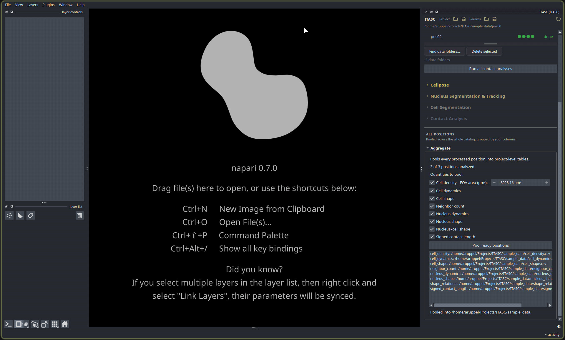
The Aggregate panel: each quantity is toggled on, Cell density additionally taking a field-of-view area, and pooling writes one CSV per quantity into the project folder, listed below the button.

Shapes and distances are reported in microns, from the pixel size set for the project.

Quantity	What it measures	Table
Cell shape	Per cell, per frame: the area, perimeter, axis lengths, aspect ratio, circularity, orientation, and related descriptors of the cell body.	cell_shape.csv
Nucleus shape	The same morphology for each nucleus.	nucleus_shape.csv
Nucleus–cell shape	Each nucleus measured against its own cell: the area and axis-length ratios between them, how far the nucleus center sits from the cell center, and the angle between their long axes.	shape_relational.csv
Cell dynamics	Per track: velocity and speed, persistence time, mean-square displacement with its power-law fit, and the tissue-scale alignment of neighboring cells.	cell_dynamics.csv
Nucleus dynamics	The same motion measures from the nucleus tracks.	nucleus_dynamics.csv
Neighbor count	Per cell, per frame: how many cells it touches, its degree in the contact graph.	neighbor_count.csv
Cell density	Per frame: the number of cells per unit field-of-view area. Requires the FOV area in square microns, set in the panel.	cell_density.csv
Signed contact length	Per T1 event: the signed length of the central junction across the swap, the reaction coordinate for its energy barrier.	signed_contact_length.csv

Where the numbers go

These tables are the end of the pipeline. The recording that entered as raw frames leaves as outlines and identities that hold across time, the graph of which cells touch and when they swap, and a set of measurements pooled across every position. What happens next, sorting cells into subpopulations, reducing to per-condition summaries, testing and plotting, is done from these tables, and is where the analysis of a particular experiment begins.